5 Easy Ways to make Spreadsheets Simple to Use

We all know that using a spreadsheet is probably not the most exciting part of running your business - let's be honest, it's more like a necessary evil. I know that you have far more important (& interesting) things to do than puzzle over a sea of numbers for hours trying to spot that nugget of information that will help you to improve your business.
What you really need is a way to make those spreadsheet simple to use and make that key bit of information really stand out so that you can see it in a flash.
If this sounds like you, then a great place to start is to add a little formatting to your spreadsheet to stop you wasting that precious time that you could be using elsewhere.
Here's 5 quick tips that you can use on any spreadsheet to make it simple to use & help you get exactly what you need from your data in the shortest possible time.
Quick Disclaimer
I use Excel for my Spreadsheets so all the images and menu options are taken from there. Most of the tips are equally applicable in other spreadsheet programmes - you just might have to dig a little to find them.
Let's start with an unformatted sheet of figures.

1. Hide Gridlines
This is so simple to do but I'm always amazed at how many spreadsheets I see (even many on sale on Etsy!) that don't do this.
Gridlines add noise to your spreadsheet and so should be hidden almost every time you create one. They add distraction and take your eye away from what you should be looking at - the information.

The one time gridlines can be useful is when you're first pulling your new worksheet together, so I suggest you first build your spreadsheet with the gridlines showing - then when you have it just about ready, hide them and see what it looks like.
You then need to move on to point 2.
2. Add Borders
So first I tell you to hide gridlines, then I tell you to add borders???
Ok, so once you've got rid of the gridlines, you will probably need to some borders back in to separate out different sections and make it easier to read your information.
The secret to remember however (as in much of life) is that less is more!
Don't replace all the gridlines you've removed with a border - just add them in where they are needed. And don't always think your borders need to be black, maybe try toning them down to gray or even use a colour.

Speaking of colour....
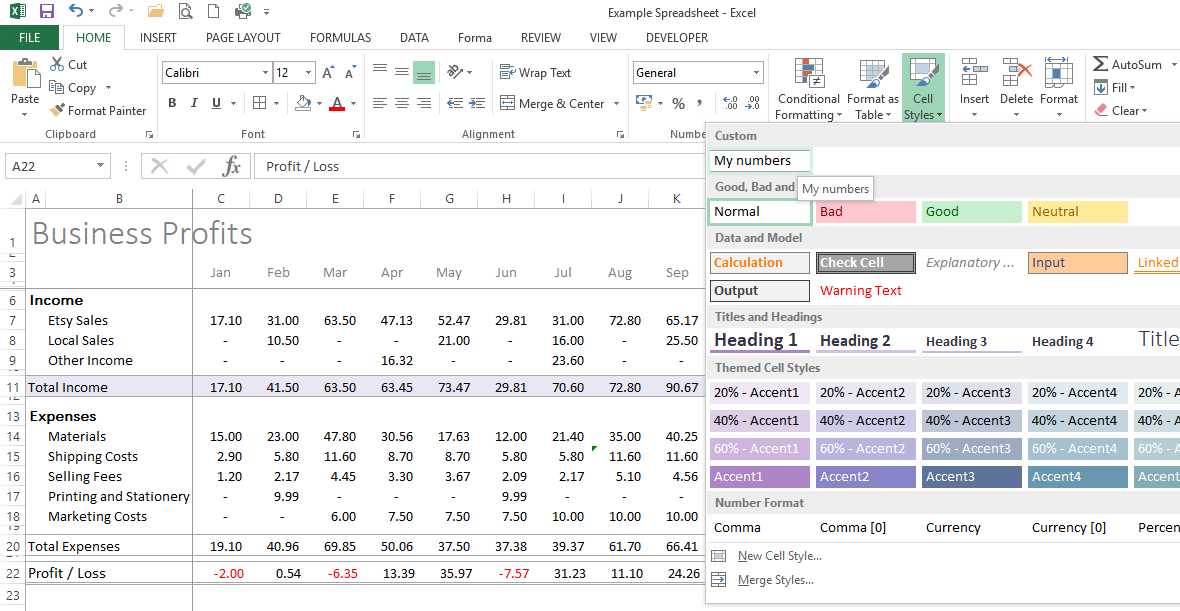
3. Use Cell Styles
This is a great quick fix that I only discovered recently (a handy reminder that you can never know it all).

Cell styles are an easy way to apply some quick formatting to a cell. Just click on your chosen cell then click cell styles & choose from the drop down selection.
Whatever you select will be instantly applied to your chosen cell ( or group of cells). Play around and try out the different styles on offer to see what they do.
Easy as Pie
BONUS TIP
Where this tool becomes really powerful is if you hit "New Cell Style" at the bottom and add some of your own. Perfect if you have a passion for orange cells with dark green font and 5 decimal places....ok maybe that's just me?
Seriously though, this is a great way to add your brand colours to your sheet.
If I'm doing a number spreadsheet (like a P&L or a sales report) that has positive and negatives, I always like my numbers to show negatives in red, so I have this set up in my cell styles.
It saves having to set it up in number formatting every time.

EXTRA BONUS
If you have some styles that you like to use a lot then the final option at the bottom of the list "Merge Styles" lets you copy your saved styles between sheets - saving you even more time
4. Use Themes
Again a pretty underused trick, but another of my favourites. It's hidden away on the "PAGE LAYOUT" ribbon so sometimes gets overlooked, but this is is a super quick way to change the look and feel of your workbook with just a couple of clicks.
THEMES let you change the default colours and fonts in your workbook to any from the dropdown lists. Just click on each of the colour options in the dropdown list and see your sheet instantly change.
Tip: This is easiest to see if you already have some colours built into your sheet. Once you start clicking down the list those coloured cells will change according to the option chosen.
Once you have made your choice it will then automatically apply to any new cells that you format.

You can do the same thing with fonts - just select any of the font combinations listed and your sheet will instantly change
Note this only works if you have used the default fonts at the top of your font list. Once you've selected a custom font from further down the list (or used one that you have added yourself) these will stay the same.
SUPER TIP
If you choose "customise" at the bottom of both colours and fonts, you can add your own options. This is a great way to bring your own style and another perfect way to keep On Brand.
EXTRA SUPER TIP
If you change the THEME, the options that appear under "CELL STYLES" will also change (but not any that you've added yourself)
5. The Format Painter
This one is super handy. Once you've spent ages getting your Theme and Cell Style just right and designed the perfectly formatted cell, you then realise that you need to do the same to all the other cells on your sheet that have similar information :-(
Before you reach for the gin (insert drink of choice here), waste hours repeating yourself or even worse give up on formatting the rest of your sheet, just click on that perfect cell and then click the FORMAT PAINTER.

Your curser will change shape to a paintbrush, and now whichever cell you click next will have the same formatting applied instantly.
This works for a group of cells as well as individual ones - even when there are different formatting styles within the group. They will all be applied to the next group you click.
Great for copying summary lines on a report.

EVEN BETTER
I only learnt this last week (after 20+ years of using Excel) but if you DOUBLE click on FORMAT PAINTER you can keep applying the formatting to every cell /group of cells you click on until you press ESC (why did I never know this!)
The ultimate time saver.
That's it
5 super easy tips to give you a beautifully designed spreadsheet with all the information you need highlighted and visible in an instant. Your worksheets will not only look more professional but far more importantly, will be much easier to use, interpret and understand.
Hide Gridlines
Add Borders to highlight key information
Use Cell Styles - to quickly add colours
Change those colours with Themes
Use the Format Painter to copy your formatting
Let me know how you get on and, even better, send me some snaps of your redesigned spreadsheets
Sarah x


Why not Pin this so you can come back to this article later?


